R FOR HERITAGE: TRAINING WORKSHOP

15 May 2019, University of Stirling

Authors: Marta Krzyzanska (marta.krzyzanska@stir.ac.uk) and Dr Chiara Bonacchi (chiara.bonacchi@stir.ac.uk)

Part 3: Data analysis

The next few sections of this training are partly based on the study published by Ben Marwick (2014), which included full documentation of the code that was used. In this study, Marwick analysed the content of the tweets containing a particular # with techniques including term frequencies, term associations, sentiment analysis and topic modelling. We further developed these analytical routines, applying them to Facebook data, as part of a study on the Heritage of Brexit (Bonacchi, Altaweel, Krzyzanska 2018).

Now, we will apply some of the techniques mentioned above to an anonymised dataset of tweets containing #hadrianswall that were extracted via streaming in 2017 and 2018. To do that, we will need the text mining library tm (the documentation for it can be found here https://cran.r-project.org/web/packages/tm/tm.pdf) and few other libraries that enable text manipulation and visualisation.

Workspace preparation

First, install all these libraries and then load them into the R workspace:

#Install the packages:
install.packages("tm")
install.packages("stringr")
install.packages("wordcloud")
install.packages("rtweet")
install.packages("rJava")
install.packages("SnowballC")
install.packages("NLP")
install.packages("pkggraph")

# Load the packages
library(tm)
library(stringr)
library(wordcloud)
library(rtweet)
library(rJava)
library(SnowballC)
library(NLP)
library(pkggraph)

Set your working directory:

setwd("/Users/yourusername/Documents/Rheritage")

Then save the .csv file containing tweets that feature #hadrianswall in your working directory and load the data into your R workspace with the following command:

d<-read.csv("data.csv")

To get an idea about the structure of the table, you can use the str() function, which is designed to show the internal structure of an R object:

str(d)

'data.frame':	4651 obs. of  22 variables:
 $ id_str                               : Factor w/ 4651 levels "anonymised_id(1001899)",..: 4288 2429 2726 2974 1702 2882 1121 4594 3548 1563 ...
 $ text                                 : Factor w/ 1810 levels "'Golden Frontier' - beautiful shot of #HadriansWall, captured by anonymised_user(6878864) at dawn today - #phot"| __truncated__,..: 470 142 702 1502 1801 701 466 1463 1125 456 ...
 $ created_at                           : Factor w/ 4645 levels "2017-09-13 09:55:54",..: 3832 4573 4607 4580 3874 4608 4561 4082 3829 4081 ...
 $ user.description                     : Factor w/ 1788 levels "","'Courage doesn't always roar. Sometimes courage is the little voice at the end of the day that says, 'I'll try "| __truncated__,..: 244 1301 95 1308 248 95 1263 1738 478 1738 ...
 $ user.followers_count                 : int  1308 86 128 4531 698 128 688 11 163 11 ...
 $ user.friends_count                   : int  959 151 591 2748 1557 591 769 46 580 46 ...
 $ user.statuses_count                  : int  2362 119 72 13651 2446 72 587 12 170 12 ...
 $ in_reply_to_status_id_str            : Factor w/ 33 levels "anonymised_id(1465387)",..: NA NA NA NA NA NA NA NA NA NA ...
 $ is_quote_status                      : Factor w/ 2 levels "false","true": 1 1 1 1 1 1 1 1 1 1 ...
 $ quoted_status_id_str                 : Factor w/ 98 levels "anonymised_id(1360931)",..: NA NA NA NA NA NA NA NA NA NA ...
 $ quoted_status.text                   : Factor w/ 99 levels "","#hadrianswall #nationaltrail around #Housesteads - you can really see the lumps and bumps of the Vicus (civilia"| __truncated__,..: 1 1 1 1 1 1 1 1 1 1 ...
 $ quoted_status.user.description       : Factor w/ 80 levels "","A collection of original illustrations, art and photography from talented local artists available as stunning l"| __truncated__,..: 1 1 1 1 1 1 1 1 1 1 ...
 $ retweeted_status.id_str              : Factor w/ 654 levels "9.39892617223e+17",..: NA NA NA NA NA NA NA NA 393 NA ...
 $ retweeted_status.text                : Factor w/ 654 levels "","'Golden Frontier' - beautiful shot of #HadriansWall, captured by anonymised_user(6878864) at dawn today - #phot"| __truncated__,..: 1 1 1 1 1 1 1 1 236 1 ...
 $ retweeted_status.user.description    : Factor w/ 190 levels "","'Give me a camera' #canon; budding #yamaha alto player, #photostreak 1090 consecutive days. anonymised_user(869"| __truncated__,..: 1 1 1 1 1 1 1 1 28 1 ...
 $ retweeted_status.user.followers_count: int  NA NA NA NA NA NA NA NA 4297 NA ...
 $ retweeted_status.user.friends_count  : int  NA NA NA NA NA NA NA NA 2486 NA ...
 $ retweeted_status.user.statuses_count : int  NA NA NA NA NA NA NA NA 4844 NA ...
 $ user.id                              : Factor w/ 1868 levels "anonymised_user(1001787)",..: 272 1308 115 1717 555 115 203 1521 873 1521 ...
 $ in_reply_to_user_id                  : Factor w/ 56 levels "","anonymised_user(1426941)",..: 1 1 1 1 1 1 1 1 1 1 ...
 $ quoted_status.user.id                : Factor w/ 74 levels "","anonymised_user(1235832)",..: 1 1 1 1 1 1 1 1 1 1 ...
 $ retweeted_status.user.id             : Factor w/ 188 levels "","anonymised_user(1065525)",..: 1 1 1 1 1 1 1 1 96 1 ...

As you can see above, the data you imported from the .csv file is a data frame consisting of 4651 observations (tweets) and 22 variables that store information about each tweet in 22 distinct columns. The names of the columns are flagged with the $ sign, and they are followed by the information about the type of data they are storing. Since the data frame is too big to visualise it in its entirety, let’s have a look at the text of the first three tweets and their creation date (respectively the second and the third columns of the data frame):

d[c(1:3),c(2:3)]

text	created_at
Hadrian's Wall. An oldie this one, and suspect there€™s more snow out there today! #hadrianswall #winter #northumberland #landscapephotography https://t.co/8NO7JzRUNs	2018-03-02 09:11:27
A sight to behold! sycamore gap, part of Hadrian€™s Wall. #sycamoregap #hadrianswall #northumberland #uk #landscapephotography #tree #sycamoretree #robinhoodprinceofthieves #payinghomage #picturesque #crowdsurfphotos #crowdsurfphotography https://t.co/U5ZdbwWVEd	2018-03-26 11:45:55
Preparing my bag for Hadrians Wall coast to coast walk. 4 weeks to go! 65L too much? #hadrianswall #hiking #Northumberland #solway #wallsend #UNICEF #hikingadventures https://t.co/QXxKY9seal	2018-03-27 12:38:05

You can have a look at any other subset of the data, by manipulating the numbers used to define relevant rows and columns or by using the names of the relevant columns.

Time series

Before we start analysing the text of the tweets, let’s get some basic and contextual information about our data. We already know, that there are 4651 tweets in the dataset.

We can also have a look at when the tweets were published. To do that, let’s inspect the created_at column more closely:

head(d$created_at)

2018-03-02 09:11:27
2018-03-26 11:45:55
2018-03-27 12:38:05
2018-03-26 16:52:02
2018-03-03 12:34:27
2018-03-27 12:40:01

This column stores the dates and times when the tweets were published, in a standardised format. We can use it to plot the time series of the tweets, using the ts_plot function from the rtweet library (a time series is a series of data points listed or graphed in a time order):

ts_plot(d, by="days")

png

As you can see above, the dataset contains tweets streamed in two separate batches. The first batch was collected between September and December 2017, and the second one in February and March 2018. Note that by stating that results should be plotted by=”days” we specified that we wanted the desired interval of time to be days.

If you want you can save the resulting plot as a .pdf, using the following command (check that the file appeared in your working directory and you can open it):

dev.print(pdf,"time_series.pdf")

Users analysis

We can also have a look at the number of unique users who posted the tweets. First, we create a variable called unique users, where we store the unique numbers corresponding to anonymised user ids, which can be obtained by using the function unique():

unique_users<- unique(d$user.id) # Function unique() returns all the unique values from the list provided as an argument.

Then, we use the length() function to get the number of unique users:

length(unique_users)

1868

There were 1868 unique users. This number is lower than the number of tweets. Let’s have a closer look at the frequency of tweets per user. To do that, let’s transform the column with the anonymised user ids into a table:

users<-table(d$user.id)
head(users)

anonymised_user(1001787)  anonymised_user(101639) anonymised_user(1019551)
                       1                        3                        1
anonymised_user(1023010) anonymised_user(1024187) anonymised_user(1024525)
                       1                        1                        1

As you can see above, the table shows the serial number corresponding to a certain anonymised user id, and the number of tweets s/he tweeted. However, this is not a very effective way of presenting data, so let’s transform the data contained in the variable users into a data frame:

users<-as.data.frame(users)
head(users)

Var1	Freq
anonymised_user(1001787)	1
anonymised_user(101639)	3
anonymised_user(1019551)	1
anonymised_user(1023010)	1
anonymised_user(1024187)	1
anonymised_user(1024525)	1

This looks better, but we also want to order users by frequency of tweeting (i.e. the number of tweets per user in the dataset), from those who tweeted less to those who tweeted more. Let’s do that and inspect the tail of the new data frame to visualise the users who tweeted the most:

users<-users[with(users,order(Freq)),]
tail(users)

	Var1	Freq
961	anonymised_user(5633442)	89
753	anonymised_user(4722486)	103
1717	anonymised_user(9224355)	124
383	anonymised_user(2851416)	136
649	anonymised_user(4223981)	142
458	anonymised_user(32252)	369

In the code above, the function with() is used to re-order the rows in the data frame (hence it is placed as the first element in the square brackets, which is used to access the rows). The with() function takes two arguments: the data by which to re-order (the data frame called users), and the function used to re-order them (in this case it is frequency, as we reorder from the lowest value to the highest). To save the table with the frequencies of the tweets per user, you can write it into a csv file:

write.csv(users, file="users_frequency.csv")

Hashtags analysis

Let’s also extract the hashtags that are present in the dataset. Knowing what hashtags are there, can give us the initial information about the themes present in our data. To extract hashtags from the text of the tweets, we will use the pre-defined str_extract_all function from the stringr library:

hashtags <- str_extract_all(d$text, "#\\w+")

This function takes as the first argument the text from which we want to extract the hashtags, and a regular expression as the second argument. This expression tells R to extract contents starting from and including # up to a whitespace (w+).

Regular expressions and functions such as str_extract_all are useful for text manipulation. If, later on, you want to have a look at the full range of text manipulation functions and regular expressions available, see https://www.rstudio.com/wp-content/uploads/2016/09/RegExCheatsheet.pdf.

Have a look at the format in which the hashtags are provided:

head(hashtags)

1. '#hadrianswall'
2. '#winter'
3. '#northumberland'
4. '#landscapephotography'
1. '#sycamoregap'
2. '#hadrianswall'
3. '#northumberland'
4. '#uk'
5. '#landscapephotography'
6. '#tree'
7. '#sycamoretree'
8. '#robinhoodprinceofthieves'
9. '#payinghomage'
10. '#picturesque'
11. '#crowdsurfphotos'
12. '#crowdsurfphotography'
1. '#hadrianswall'
2. '#hiking'
3. '#Northumberland'
4. '#solway'
5. '#wallsend'
6. '#UNICEF'
7. '#hikingadventures'
1. '#hadrianswall'
2. '#Hadrianswall'
1. '#Snow'
2. '#RomanPower'
3. '#HadrianWall'
4. '#Roman'
5. '#Britain'
6. '#Arrago'
7. '#Mansio'
8. '#AquaCalidae'
9. '#Iesso'
10. '#Tarraconensis'
11. '#Barcino'
12. '#Baetulo'
1. '#hadrianswall'
2. '#hiking'
3. '#Northumberland'
4. '#solway'
5. '#wallsend'
6. '#UNICEF'
7. '#hikingadventures'

The texts were originally provided as a vector, and the extracted hashtags are also returned as a vector.

As you can see, each element in this vector, contains a vector of hashtags that appeared in a given tweet. To simplify this vector of vectors into a simple list of hashtags, we can unlist it and have a look at the first few #:

hashtags<-unlist(hashtags)
head(hashtags)

'#hadrianswall'
'#winter'
'#northumberland'
'#landscapephotography'
'#sycamoregap'
'#hadrianswall'

Now we have a simple list of all the hashtags that appear in the tweets. Let’s find out how many times a # was used and how many unique hashtags there are in the tweets:

length(hashtags)
length(unique(hashtags))

11577

882

##### Q1.Try to make a frequency table for hashtags. Which hashtags feature most frequently? The code you can use to produce the table is given at the end of this tutorial.

Document-term matrix

In this section, we will take a closer look at the content of the tweets. To do this, we will transform the texts of the tweets into a document-term matrix. This is a special type of data structure which stores the texts of the tweets in a way that allows them to be easily queried and analysed.

First, extract the texts from the data frame and store them as a simple vector of texts:

texts<-iconv(d$text)

# d$text is wrapped in the iconv() function, which transforms the utf-8 enconding into a format readeble by R.
# in most cases it is not needed, but if you encounter errors related to utf-8 encoding, simply use this function.

head(texts)

Hadrian€™s Wall. An oldie this one, and suspect there€™s more snow out there today! #hadrianswall #winter #northumberland #landscapephotography https://t.co/8NO7JzRUNs
A sight to behold! sycamore gap, part of Hadrian€™s Wall. #sycamoregap #hadrianswall #northumberland #uk #landscapephotography #tree #sycamoretree #robinhoodprinceofthieves #payinghomage #picturesque #crowdsurfphotos #crowdsurfphotography https://t.co/U5ZdbwWVEd
<span style=white-space:pre-wrap>Preparing my bag for Hadrians Wall coast to coast walk. 4 weeks to go!\n65L too much? #hadrianswall #hiking #Northumberland #solway #wallsend #UNICEF #hikingadventures https://t.co/QXxKY9seal</span>
The Hadrianic bath house at Chester€™s Fort sits next to #hadrianswall on the North Tyne river extended over time with heavy buttressed latrine #Hadrianswall https://t.co/rcJsn7f5nw
Winter on Hadrian's Wall. How did Romans cope with snow? \nhttps://t.co/g0ZtEDO3Te\n#Snow #RomanPower #HadrianWall #Roman #Britain #Arrago #Mansio #AquaCalidae #Iesso #Tarraconensis #Barcino #Baetulo https://t.co/h4nSJRTrW4
<span style=white-space:pre-wrap>Preparing my bag for Hadrians Wall coast to coast walk. 4 weeks to go!\n65L too much? #hadrianswall #hiking #Northumberland #solway #wallsend #UNICEF #hikingadventures https://t.co/2WPcSfRROP https://t.co/3nYYjGamwF</span>

Then, transform the texts into a corpus. A corpus is a collection of documents (in our case each tweet is a document) that can be read and manipulated using the tm library:

a <- Corpus(VectorSource(texts))
#interpret all elements of the vector composed of texts as a document and create a corpus with those documents.
a

<<SimpleCorpus>>
Metadata:  corpus specific: 1, document level (indexed): 0
Content:  documents: 4651

Now that we have a corpus of tweets, let’s use the tm library to clean our textual data and prepare it for the analysis. We will use tm_map, which is an interface useful to apply transformation functions to corpora. First, we will modify all the words in the corpus so they are in the lowercase:

a <- tm_map(a, tolower)
#here the tm_map interface is used together with the function tolower() to change all terms to the lowercase

Get rid of all punctuation:

a <- tm_map(a, removePunctuation)
#here the tm_map interface is used together with the function removePunctuation() to remove punctuation from the documents

Remove numbers:

a <- tm_map(a, removeNumbers)
#here the tm_map interface is used together with the function removeNumbers to remove all the numbers from the documents

Remove English stopwords. Stopwords are those words that are not particularly meaningful on their own, in a certain language. Examples of English stopwords are: “a”, “the”, “in”.

a <- tm_map(a, removeWords, stopwords("english"))
#here the tm_map interface is used together with the function removeWords to remove English stopwords
#function stopwords produces the list of stopwords in the language specified as an argument
#you can use this function also to remove other words that may create noise in the data

Finally, stem all the words in the corpus. Stemming is a procedure used to remove word endings and ensure that only the root of a word is retained. This leaves us with ‘a single token that indicates different forms of the same word that have a common meaning’ (Marwick 2014: 83):

a <- tm_map(a, stemDocument, language = "english")
#here the tm_map interface is used together with the function stemDocument() to tokenize words

Now the corpus is ready to be transformed into a document-term matrix (dtm). In this case, during the transformation we want to keep only the tokens that are longer than 3 letters:

dtm  <- TermDocumentMatrix(a, control = list(minWordLength = 3))
# (minWordLength = 3) means that the minimum length of the terms we are keeping is 3 letters

Inspect the dtm to get an idea of how the data is structured:

inspect(dtm[1:10,1:10])
#inspect() allows you to 'display detailed information on a corpus, a term-document matrix, or a text document'
# [1:10,1:10] allows you to specify that you want the first 10 terms and 10 documents to be displayed

<<TermDocumentMatrix (terms: 10, documents: 10)>>
Non-/sparse entries: 26/74
Sparsity           : 74%
Maximal term length: 20
Weighting          : term frequency (tf)
Sample             :
                      Docs
Terms                  1 10 2 3 4 5 6 7 8 9
  hadrianÃ             1  0 1 0 0 1 0 0 0 0
  hadrianswal          1  1 1 1 2 0 1 1 1 1
  httpstconojzrun      1  0 0 0 0 0 0 0 0 0
  landscapephotographi 1  0 1 0 0 0 0 0 0 0
  northumberland       1  0 1 1 0 0 1 2 0 0
  oldi                 1  0 0 0 0 0 0 0 0 0
  one                  1  0 0 0 0 0 0 0 0 0
  snow                 1  0 0 0 0 2 0 0 0 0
  suspect              1  0 0 0 0 0 0 0 0 0
  thereÃ               1  0 0 0 0 0 0 0 0 0

In the document-term matrix, each row is a different term that appears in the corpus and each column is a different document contained in the corpus. The numbers indicate how many times a certain term appears in a certain document.

Term frequencies

Now we can start carrying out some simple analyses on our dtm. First, let’s find out what the terms with the highest frequency (those that recur the most) are, by using the function findFreqTerms():

findFreqTerms(dtm, lowfreq=400)
#Get the terms that feature at least 400 times

'hadrianswal'
'northumberland'
'wall'
'roman'
'nationaltrail'
'anonymisedus'
'along'
'crag'
'morn'
'archaeolog'

Now, let’s get the terms that feature between 200 and 400 times:

findFreqTerms(dtm, highfreq=400,lowfreq=200)

'today'
'hadrian'
'walk'
'fort'
'mile'
'found'
'day'
'lough'
'section'
'housestead'
'milecastl'
'near'
'beauti'
'romanbritain'
'frontier'
'vindolanda'
'hadrianswallÃ'
'westtoeast'

And the terms that feature between 100 and 200 times:

findFreqTerms(dtm, highfreq=200,lowfreq=100)

'one'
'snow'
'hadrian'
'north'
'time'
'build'
'amp'
'love'
'nlandnp'
'view'
'weather'
'trigpoint'
'stone'
'see'
'great'
'histori'
'built'
'walltown'
'just'
'want'
'new'
'good'
'steel'
'show'
'now'
'sewingshield'
'still'
'altar'
'look'
'can'
'turret'
'ditch'
'head'
'carlisl'
'west'
'light'
'scene'
'httpsÃ'
'snowi'
'inÃ'
'httpstcÃ'
'hotbank'
'misti'
'crisp'
'excav'
'autumn'
'fine'
'frosti'

As you can see, the most frequent terms largely overlap with the most frequent hashtags, but there are also other tokens associated for example with weather, excavations and archaeological sites.

Term associations

To start exploring quantitatively the context in which these frequently recurring terms feature, we can have a look at the terms that are most strongly associated with them. For example to find associations for the term ‘frontier’ type:

findAssocs(dtm, "frontier", 0.30)
#find terms that are associated with the term 'frontier', with correlation >0.3

$frontier =

golden: 0.8
northernmost: 0.8
dawn: 0.79
break: 0.76
empir: 0.69
httpstcopaÃ: 0.49
inÃ: 0.46
scene: 0.4
snowi: 0.4
roman: 0.36
romanbritain: 0.33

Try inspecting different terms. The number given in the formula above (0.3), indicates the minimum strength of correlation between the terms in the corpus of documents (i.e. how often they occur together) and can vary between 0 and 1. You can adjust this number as necessary (the lower the number, the lower the minimum strength of the association, and the more terms will be displayed).

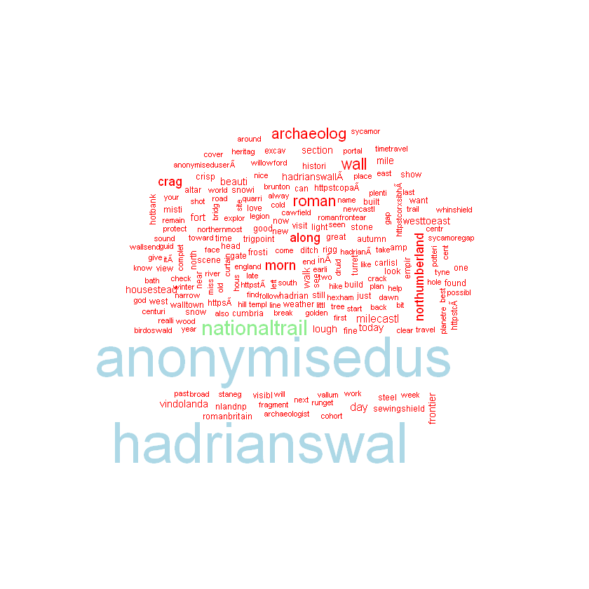
You can also display the corpus of texts as a word cloud and save it in your workspace:

wordcloud(a,max.word=200,colors=c("red","lightgreen","black","lightblue"))
dev.print(pdf,file="terms_wordcloud.pdf")
#create a word cloud from the corpus (a)
#it will have a max of 200 words
#to create the word cloud, use the colours red, lightgreen, black, lightblue
#then save the wordcloud to your workspace

png: 2

png

Finally, save your document-term matrix as an R object:

save(dtm,file="dtm.R")

We can also create and inspect the document-term matrix from the description of the user profiles. To do this, first get unique user descriptions and store this data in the user_desc variable:

users_desc<-unique(d$user.description)

Q2. Create a document-term matrix from user descriptions and explore the data as we have done above.

The code is given at the end of this tutorial.

**The operations of manipulations and data analysis we have seen are a good springboard for more sophisticated quantitative analysis such as cluster analysis, topic modelling and social network analysis. They are also a really useful way to explore the content of large data sets and make decisions on what to analyse qualitatively and how. **

Well done! You have reached the end of the training. We hope you enjoyed it and found enough food for thought.

Solutions

Q1: Try to make a frequency table for hashtags. Which hashtags feature most frequently?

hashtags<-table(hashtags)
hashtags<-as.data.frame(hashtags)
hashtags<-hashtags[with(hashtags,order(Freq)),]
tail(hashtags) ## remember that the tail() function allows you to visualise the last few rows of a dataset.

	hashtags	Freq
560	#Northumberland	333
335	#Hadrianswall	334
42	#Archaeology	399
521	#nationaltrail	1217
336	#HadriansWall	1591
333	#hadrianswall	2354

Q2: Create a document-term matrix from user descriptions and explore the data as we have done above.

a <- Corpus(VectorSource(users_desc))
a <- tm_map(a, tolower)
a <- tm_map(a, removePunctuation)
a <- tm_map(a, removeNumbers)
a <- tm_map(a, removeWords, stopwords("english"))
a <- tm_map(a, stemDocument, language = "english")
dtm.users  <- TermDocumentMatrix(a, control = list(minWordLength = 3))
save(dtm.users,file="dtm_users.R")

findFreqTerms(dtm.users, lowfreq=100)
findFreqTerms(dtm.users, lowfreq=50, highfreq=100)

'archaeolog'
'histori'
'love'

'photograph'
'follow'
'photographi'
'life'
'archaeolog'
'interest'
'wall'
'time'
'world'
'writer'
'live'
'northumberland'
'book'
'walk'
'travel'
'roman'
'author'
'lover'
'art'
'artist'
'music'
'tweet'
'anonymisedus'
'view'
'work'
'write'
'fan'
'\u0081'

References

Bonacchi, C., Altaweel, M., Krzyzanska, M. (2018) The heritage of Brexit: Roles of the past in the construction of political identities through social media. Journal of Social Archaeology 18(2): 174-192. DOI: 10.1177/1469605318759713.

Marwick, B. (2014) Discovery of Emergent Issues and Controversies in Anthropology Using Text Mining, Topic Modeling, and Social Network Analysis of Microblog Content. Data Mining Applications with R. Amsterdam: Academic Press, Elsevier, pp. 63-93.

Stirling R for Heritage Training Workshop